The Technology of NLBS(Non-Performing Loan Bid System)
The technology provided here enables to match these people who want to sell a loan and those people who want to purchase a loan.
The technology consist Non-Performing Loan Bid Market itself, which functions among economic units on net market.
Ⅰ Input Items for Deal
The followings are the seller’s input data as deal conditions. These data are the items of the deal.
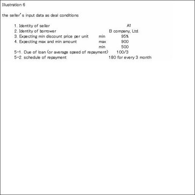
1. The identity of the seller. Usually specified by name and it’s location.
2. The identity of the borrower. Usually specified by name and it’s location.
3. Maximum(hereinafter referred to as “max”) and minimum(hereinafter referred to as “min”) amount
4. Min discount price per unit
5. Due of loan(schedule of repayment, or average speed of repayment)
The followings are the purchaser’s input data as deal conditions. These data are also the items of the deal.
1. The identity of the purchaser. Usually specified by name and it’s location.
2. The identity of the borrower. Usually specified by name and it’s location.
3. Max and min amount
4. Max discount price per unit
5. Due of loan(schedule of repayment, or average speed of repayment)
Ⅱ Two Phases that Consists Deal
The process of deal is divided into two phases, first for seeking operation and second for bidding operation.
Seeking operation process is needed because by changing the input data by seller and by purchaser, seller and purchaser can seek and find out the whereabouts of counterpart’s conditions.
It’s a presupposition that the purchaser’s debt, which will be offset by the loan when acquired in the bidding operation, is fixed and will not be assigned, once after the purchaser enter the aforesaid bidding operation, till aforesaid bidding operation is over.
Ⅲ Functions of NLBS
Here, the basic functions of NLBS concerning above items is shown.
1. Max and Min Amount
NLBS can show the max and min amount that seller and purchaser want to sell or purchase at this seeking operation.
NLBS select and display to seller the amount which exceeds the seller’s min amount input by purchaser, and so do NLBS to seller the amount which is within the seller’s max amount input by purchaser. NLBS select and display to purchaser the amount which exceeds the purchaser’s min amount input by seller, and so do NLBS to purchaser the amount which is within the purchaser’s max amount input by seller.
In general, it’s possible to subdivide the amount of loan. And it’s also possible to integrate the amounts of loans. Illustration 1 is the logic for NLBS to show the possible deal between sellers and purchasers.


2. Discount Price per Unit
NLBS select and display to seller the discount price per unit which exceed the seller’s min discount price per unit input by purchaser, and so do NLBS to purchasers the discount price per unit which is within the purchaser’s max discount price per unit input by seller.
Seller and purchaser can decide the max and min discount price per unit they want to sell or purchase.
Illustration 2 is the logic for NLBS to show the possible deal between seller and purchaser.
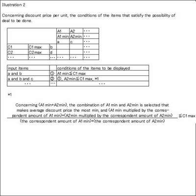
 Several sellers and purchasers who satisfy the equation Amin≦Cmax in average discount price per unit have the possibility for deal.
Here, we see how average min discount price per unit is calculated among two sellers A1 and A2 for single purchaser C1. This is the case *1 of ② on illustration 2.
As there exists two sellers A1 and A2, so each of them offers it’s own min discount price per unit.
Furthermore, let me explain by putting here an example as follows: A1min<A2min in discount price per unit, in amount A1min=90, A1max=100, in amount A2min=70, A2max=110, and in amount C1min=170 C1max=230. The detail is illustrated on illustration 3, on three dimension coordinates.
 First, the amount of the most min discount price per unit A1 is used till max 100(illustrated by solid line α), and then the amount of next most min discount price per unit A2 is used till 70(illustrated by solid line β). That makes 170, which A1min+A2min is the most min in discount price per unit. In this case, dealing should be done in amount from 170 to 210.
3. Speed of Repayment
NLBS can select, package and display the due and the amount of the seller that exceeds the speed of repayment input by purchaser. The sellers’ input of the exact schedule of each loan makes this possible. The logic is on Illustration 4.
 Let me explain further. Illustration 5 shows the average pitch of repayment which B owes to A.Straight line a, b and c show the average speed of repayment till max.
 The sharper the slope is, the faster the speed of repayment till max amount is. If the conditions of amount and discount price per unit are the same, the sharper the slope is, the more value the sharper slope has. The display by NLBS for straight line a is 100/3, for b is 100/9 and for c is 100/15.
NLBS hold the complete data of repayment schedule, therefore NLBS is able to display the required due. On illustration 5, straight line a, b and c show the average term needed to repay till max amount. In fact, for straight line c, the real repayment is sometimes curved as d or e. Let me put an example here as follows: When A1 hold loan 100 to B1, repayment speed is c but in fact the real repayment schedule is d, and A1 intend to sell in amount A1max=100, A1min=80. On the other hand C1 intend to purchase loan in amount C1max=80 and at repayment speed 100/12. In this case NLBS can show the point α to C1 on curbed d(in this case the repayment speed of the remainder is more flat, and it’s repayment start later than 9 month). On curbed e case, there is no point that NLBS can show to C1.
Ⅳ The Number of Participants
Regardless of any borrower, the number of participants changes for each side, according to the stage of bidding
In the early stage of dealing, there exists only purchasers’ offer. In the next stage, there comes the first seller’s offer. This process occurs in seeking operation. The first seller is to set up the first bidding operation of her or his own, and execute the bidding. The bidding is basically set up accordingly to each seller’s timing to enter the market. It’s up to each purchaser, whether she or he participate in the first bidding or wait till the next bidding by another seller.
Ⅴ Dealing Process
Let me put you in a picture of dealing process.
After the seller input the items of the deal, the seller’s display is as illustrated 6.
 At the seeking operation, the display for the seller is as illustrated 7.
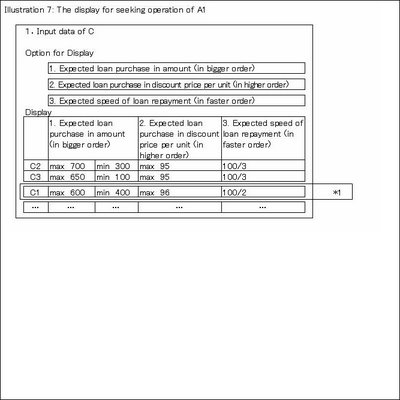
 These Cs that match the seller’s input conditions are displayed. In this case, C2 and C3 are displayed. When A1 alters the pitch of repayment from 100/3 to 100/2 in 3, C1 is newly displayed.
After the purchaser input the elements of the deal, the purchaser’s display is as illustrated 8.

At the seeking operation, the display for the purchaser is as illustrated 9.

 The A2 that match the purchaser’s input conditions are displayed. In this case, when C1 alters the pitch of repayment from 100/2 to 100/3 in 3, A1 is newly displayed.
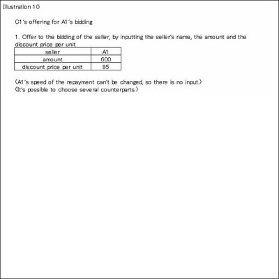
On illustration 10, C1 is offering to A1’s bidding. After all offers are done on bidding date, the highest bid price wins the bidding.
The Economic Model 2
The formula and the way to measure offset multiplier effect through NLBS are provided on this post.
Concerning the real B/S of B, next equation can be quoted.

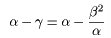
The ratio represents the real value of the loan held by A to B(β≦α). The price which C should pay to purchase loan from A is γ, which compose next equation. This procedure is necessary to measure following multiplier effect.

In this case multiplier effect(=α-γ) is as follows(formula1):
Next, concerning the real B/S of D, there exists the amount δ, which leads to next equation. The price which E should pay to purchase loan from C is γ. It is known that in fact the purchase price is not always γ, but it is permitted because if the deal should not been done, or if there exist the remainder, these offset profit will be taxed and absorbed by the government(when consecutive deal is done at γ2, (γ2-γ)will be taxed all). Usually γ consist the part of the payment to purchase next loan(in case deal is done at γ1, (γ-γ1)is supplemented by internal reserve of the economic unit). Please see figure 1, too.

In this case multiplier effect (=β-γ) is as follows(formula2):


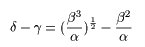
And so, concerning the real B/S of F, there exist the amount ε, which leads to next equation.

In this case multiplier effect (=δ-γ) is as follows(formula3):
In conclusion.
For each distribution, there exist each amount, which is expressed by next equation in general, for n≧3:

And for multiplier effect. We find next reccursive formula, for n≧4(formula4):

We can calculate the offset multiplier effect as on figure 2.

In general, for multiplier effect, next formula is quoted for n≧3:

In case of reverse wealth effect, as on the economic model edited on this blog June 09, 2005, the central bank can pass through the initial fund(=α-γ) to A and distribute to other economic unit. It is different from money supply. The central bank should play this role, as well as lender of last resort or provision of liquidity. Because every economic unit act based on both the real balance sheet and the expectation for the real balanace sheet, both are to be reformed through NLBS, by the central bank. There might be the case that the value lost in asset depreciation been covered to some extent by the initial fund provided by the central bank and it's multiplier effect, should there been no fear of inflation. This may leads to an equilibrium point in economy. Consequently the equilibrium point may be realized by the work of central bank as mentioned above. And as you can see on figure 2, it must be remarked that the earlier the central bank take action, the bigger the multiplier effect of initial A will be.
The Economic Model
Here is the economic model:
Every economic unit holds credits(assets) to other economic units, which relations that bring income to the former. The credit(assets) held by the economic unit is the debt(liability) carried by the other economic unit, and the debt(liability) carried by the economic unit is the credit(asset) of the other economic unit. When the credit and the debt take time to be settled, the value of the credit is appraised based on the debtor's current value accounting. The current value accounting of the economic unit is defined as the appraisal of the face value of the balance sheet(B/S) into current market value and it's reflection to the income statement(P/L). Those economic units who can maintain profit on the P/L continue to exist and those economic units who can not maintain profit go into liquidation. In recession(yield downward, money supply decreased, price deflation), generally many economic units reckon up the losses on the P/L. Furthermore, loss inflicted by assets deflation and with the effect multiplied by current value accounting, incur "spiral of insolvent" on quite a few economic units. We look over this phenomenon in the simplified case as follows:
Five economic units from A to E are abstracted among all economic units in the economy. Economic unit A holds loans for B(B carries loan payable to A), so does B for C, so does C for D, so does D for E, so does E for A for the face value, and each economic unit hold assets such as real estate for the face value(stated immovable account) as below.
Figure 1
B/S of A| Loan 100 | Loan Payable 100 |
| Immovable a/c 100 | Loan Payable 100 |
B/S of B| Loan 100 | Loan Payable 100 |
| Immovable a/c 100 | Loan Payable 100 |
B/S of C| Loan 100 | Loan Payable 100 |
| Immovable a/c 100 | Loan Payable 100 |
B/S of D| Loan 100 | Loan Payable 100 |
| Immovable a/c 100 | Loan Payable 100 |
B/S of E| Loan 100 | Loan Payable 100 |
| Immovable a/c 100 | Loan Payable 100 |
After fiscal(one) year, we assume the earnings of each economic unit is as below.
Figure 2
During the same fiscal year, assets deflation occurred and the face value of the real estate is revaluated from 100 to 96, on each economic unit as below.
Figure 3
Concerning from A to E, we put two assumptions here. First, before the start of aforesaid fiscal year, due to asset deflation, the valuation of assets is so down for assets section to equal liability section (that is, on B/S the value of stockholders' equity section came to zero). Second, in appraising the loan by current value accounting of each economic unit, the total amount of earning(or loss) of the debtor must be divided by all the loan amount held by it's creditors, and we assume half the amount is the loan appraisal loss reckoned up on a single creditor. Hereinafter, we always apply this assumption to each economic unit. We must note that the same phenomenon occurs to the rest half. So, the loan held by A for B, asset deflation inflicts B for 4 and loss distress B for 4 so in total loan appraisal loss will be 8, and half the amount 4 is the loan appraisal loss reckoned up on A. The loan, held by B for C, though asset deflation inflicts C for 4, C earned 5 so no loan appraisal loss is to be reckoned up on B. The loan, held by C for D, D suffers Loss 6 and assets deflation 4 for total 10, so half the amount 5 is reckoned up as loan appraisal loss on C. The loan, held by D for E, though E suffers asset deflation 4, E earned 1, in summing up 3, so D reckons up half the amount 1.5 as loan appraisal loss. The loan, held by E for A, though asset deflation inflicts A for 4, A earned 4 so no loan appraisal loss on E(Phase Ⅰ). Each economic units' loan appraisal loss is as below.
Phase Ⅰ
P/L of A| Loan Appraisal Loss 4 | |
P/L of B| Loan Appraisal Loss 0 | |
P/L of C| Loan Appraisal Loss 5 | |
P/L of D| Loan Appraisal Loss 1.5 | |
P/L of E| Loan Appraisal Loss 0 | |
And then, it moves on to next phase. E reappraises the loan for A by taking into account A's loan appraisal loss 4, and reckon up half the amount 2 as reappraisal loss. D reappraises the loan for E by taking into account the loan reappraisal loss 2 on E and reckons up half the amount 1 as reappraisal loss. C reappraises the loan for D by taking into account the loan appraisal loss 1.5 and loan reappraisal loss 1, in total 2.5, reckoning up half the amount 1.25 as loan reappraisal loss. B reappraises the loan for C by taking into account the loan appraisal loss 5 and loan reappraisal loss 1.25, in total 6.25, reckoning up half the amount 3.125 as loan reappraisal loss. A reappraises the loan for B by taking into account the loan reappraisal loss 3.125 on B and reckons up half the amount 1.5625 as loan reappraisal loss. And it circulates again. This proceeds lasts and spirally inflict the B/S of each economic unit as multiplier effect(Phase Ⅱ), and cause another asset deflation. This is "spiral of insolvency". Every single economic unit acts rationally, but on the whole economy fall into the fallacy of composition.
The spiral of insolvency is curbed by sufficient internal reserve that certain economic units hold. But in the possible case, spiral of insolvency is more effective to depress the economy than that, or the stimulation of the economy by lower rate or public investment. In that case there is little chance for the economy to recover. Perhaps it is difficult to tell the way how, and the extent to which, current value accounting affect economy under asset deflation.
Phase Ⅱ
P/L of A| Loan Appraisal Loss 1.5625 | |
P/L of B| Loan Appraisal Loss 3.125 | |
P/L of C| Loan Appraisal Loss 1.25 | |
P/L of D| Loan Appraisal Loss 1 | |
P/L of E| Loan Appraisal Loss 2 | |
For this solution, Non-Performing Loan Bid System(hereinafter called "NLBS″) is necessary. Next, we look how NLBS basically functions among economic units X, Y and Z. NLBS's site is provided on net market. There are X1, X2, ・・・Xn who want to sell loan for Y1 at discount price, as Y1 is insolvent based on current value accounting. On the other hand there are Z1, Z2, ・・・Zn who want to buy loan for Y1, and offset it's debt to Y1. In this situation X1, X2, ・・・Xn and Z1, Z2, ・・・Zn input data of deal conditions(1)(discount price, amount, due et al. Generally the earlier the due is, the higher the price). Then the counterpart is found that most matches the conditions, and the deal done(2). The loan is assigned from X1 to Z1(3). Z1 disclaim the benefit of term of loan payable to Y1 and offset at face value, which leaves gains to Z1. Z1 pay to X1 for the price and immediately after the receipt by X1 the fund is deposited to escrow account(4). The fund remains in escrow account in the name of X1 and Z1(joint account) for certain period, until no chance exists for offset to be avoided(the term is to be politically variable), as right in act of Y1's bankruptcy, and then the fund is to be released finally to X1. Both assignment and offset are advised to Y1(5). In the case the offset is avoided as right in act of Y1's bankruptcy, the status quo ante is restored, and the fund is returned to Z1.
NLBS is a non-performing loan trading market itself. As NLBS function to adjust the B/S of Y1, it pressures Y1 to leave the market where Y1 stays now, and in fact, it forces to leave. To avoid driven out of the market, Y1 must take measures to dissolve the insolvency, by increasing capital, by debt-for-equity-swap, or by realizing enough profits, et al.
Figure 4
| Seller X1 | -data input(1)→ | Net Site | ←data input(1)- | Buyer Z1 |
| -deal(2)→ | ←deal(2)- |
| ―――――――――assign loan(3)――――――――→ |
| ←―――――――――payment(4)――――――――― |
| ―assign notice(5)→ | Y1 | ←―offset notice(5)― |
| ↓deposit(4) |
| Escrow Account |
NLBS works to improve the B/S of the economic units together with economic policy of government and central bank, in recession. Now we look at this:
We add central bank and bank to the aforesaid economic units. Bank holds loan for A. Bank's debenture or certificate deposit(CD) which the central bank have purchased beforehand for face value 100, is to be assigned to A(illustrated in red letter in later figure) found through NLBS, in the deal who offered the highest price 95. Because the deal between central bank and A is made as economic policy, authorities must declare that the deal is irrelevant to the corporate credit ratings of the bank. A offset the face value of the CD and the loan payable to bank. A assign the loan for B to C(illustrated in blue letter in later figure), and C offset the face value of the loan and debt. C assign the loan for D to E(illustrated in orange letter in later figure), and E offset the face value of the loan and debt. The initial offset gains provided to A bring about offset gains to C for 4 and E for 4, which make 12 "offset multiplier effect" in all. A and C don’t need to reckon up additional reappraisal loss because it disposed of non-performing loan. If E do not or can not find counterpart through NLBS, the offset gains remained on E will be charged tax,till the same amount, which becomes another fund to cause offset multiplier effect again. The offset gains and assigned loss are summed up, and exempt tax as a system(4 for A and 4 for C). The chance also exists for B and D to improve their B/S. As a whole, the situation phaseⅠ to move on further to phaseⅡ is avoided.
Figure 5
B/S & P/L of Central bank| CD 100 | |
| Cash 95 | CD 100 |
| Assign Loss 5 | |
B/S of Bank| Loan 100 | CD 100 |
B/S & P/L of A| Loan 100 | Loan Payable 100 |
| CD 100 | Cash 95 |
| Offset Gain 5 |
| Loan Payable(offset)100 | CD(Offset) 100 |
| Cash 96 | Loan 100 |
| Assign Loss 4 | |
B/S of B| Loan 100 | Loan Payable 100 |
B/S & P/L of C| Loan 100 | Loan Payable 100 |
| Loan 100 | Cash 96 |
| Offset Gain 4 |
| Loan Payable(offset)100 | Loan(Offset) 100 |
| Cash 95 | Loan 100 |
| Assign Loss 5 | |
B/S of D| Loan 100 | Loan Payable 100 |
B/S & P/L of E| Loan 100 | Loan Payable 100 |
| Loan 100 | Cash 95 |
| Offset Gain 5 |
| Loan Payable(offset)100 | Loan(Offset) 100 |
As a result:
For A: disposal of non-performing loan completed, offset multiplier effect 4, offset gains 1 taxed all
For C: disposal of non-performing loan completed, offset multiplier effect 4, no tax to offset gains 0
For E: no non-performing loan, offset multiplier effect 4, offset gains 4 taxed all
The establishment of the NLBS means to acquire new channel for the government and the central bank to cope with B/S recession, which derived from B/S adjustment. The initial gains provided to the first economic unit by central bank diffuse to the other economic units, through NLBS, bringing about offset multiplier effect. The gains works like a catalyzer. Through the disposal of non-performing loan on economic units concerned, it directs assets to exceed debts substantially on B/S. Offset multiplier effect can cope with the case that spiral of insolvent is more effective to depress the economy than the curb by sufficient internal reserve that certain economic units hold, or the stimulation of the economy by lower interest rate or public investment. Because offset multiplier effect works directly to the B/S of economic units, it stimulates the economy together with lower interest rate or public investment, and it enables government to bring more effectiveness for less expenditure. NLBS must be put in operation before the majority of economic units become insolvent, and before the extent of insolvent become terrible.
Before and After Real Estate Bubble In Japan
I would like to tell what I saw before and after the real estate bubble in Japan.
In Japan, banks were the biggest player to pour money into real property. Bank made loans to firms and to individuals on real estate collateral basis. To make matters simple, I would like to say that there were no Fannie Mae or Freddie Mac, and no mortgage market in those days in Japan.
Under the bubble, the return of investment on real estate from initial payment till future capital gain together with fruit born(accrued from rent, and so on), can be measured by “yield”. Demand for loan raised rate, and so long as expectations exist for the “yield” to exceed the expected rate, the investment to real estate continued and the bubble won’t burst (even Central Bank tightened its’ monetary policy). The hike in the market of real estate brought wealth effect to the economy.
Not all people were happy about the hike, because for the people who came late to real estate market felt opportunity unequal.
There were no means but to factitiously put down the price of real estate.
The policies established by the authorities concerned were as follows:
1) The principle that real estate must be purchased for the purpose of ultimate utilization, not for speculation
2) The principle that real estate should be transacted at appropriate price, not at speculative price
3) The restriction on quantity of loan to each bank on developing real estate, which become collateral for the bank.
4) The duty to each bank to strictly confirm the purpose of loan before executing, if it is for ultimate utilization or not.
5) Capital gain taxed heavily to the possessor, if the term between real estate purchased and sold is short
6) Unoccupied land (=undeveloped land or land without any utilization) which satisfied certain conditions, taxed heavily.
These policies succeeded in amending above expectations, and in fact, real estate price did begin to fall. But it caused another problem.
Till then quite a few firms and individuals possessed real estate, so the drop on the price of real estate directly inflicted their balance sheet. Moreover, the trend to appraise balance sheet on market price basis (under the situation, only fruit born against initial payment is grasped as “yield”, when appraising the real estate) brought about many insolvent firms. The way to protect their balance sheet was to sell real estate and to repay loan to bank as soon as possible, which spur the drop on the price of real estate and caused rate to dive as much money were supplied to the market. Some firms couldn’t avoid bankruptcy and damaged the balance sheet of the banks, some of which bankrupted too.
During these period, public investment and private companies’ export on depreciated yen bolstered GDP. As a consequence, the government comes to hold the worst fiscal deficit among the government in developed country, interest rate pegged at practically zero level and the depreciated yen favors some export companies and export manufacturers.
Later, the above policies were gradually abolished, but left durable balance sheet adjustment on the economy. It seems many companies that are unlisted on stock market are still groaning under huge debt on their balance sheet.
We can learn from this fact that, impressing expectation that above “yield” is lower than the above rate, incurs asset depreciation and further incurs balance sheet adjustment that exceeds the effect of fiscal policy and monetary policy.To avoid the situation, certain system must be built in the society beforehand.
